Methodology
This research package contains three complete analysis pipelines for the strongest testable predictions of the sub-quantum grid model. Each pipeline is executable against existing public data — no new experiment needs to be set up.
| # | Prediction | Data source | Script | Plot |
|---|---|---|---|---|
| 17 | Helix-resonance peaks in pair production | CERN Open Data / HEPData | prediction17_pair_production.py | below |
| 15 | Planck-scale anisotropy (grid lattice) | Fermi-LAT GRB catalog | prediction15_fermi_lat.py | below |
| 18 | Non-linear Shapiro delay | NANOGrav / NICER | prediction18_pulsar_timing.py | below |
All scripts run on Python 3.8+ with numpy, matplotlib, and scipy.
Prediction #17 — Helix Stability Threshold in Pair Production
Core hypothesis
Pair production (γ → e⁺e⁻) shows resonance peaks at harmonics of 2 m_e c² = 1.022 MeV.
The peaks have a Breit-Wigner profile and decay as 1/n² with harmonic number n.
Why this is the sharpest test
QED predicts the pair-production cross-section to 8+ decimal places of accuracy. Any deviation, however small, would be a fundamental discovery. Moreover: the resonance peaks at harmonics are a unique prediction of the grid model — no other framework predicts peaks at exactly these energies.
Required data
- Pair-production cross-section measurements near threshold (1–10 MeV)
- CERN Open Data: LEP / OPAL / DELPHI datasets
- HEPData: published cross-section tables
- Ideally: high-resolution energy scans (ΔE < 0.05 MeV)
Required statistics
| Signal amplitude | 3σ detection requires | Feasibility |
|---|---|---|
| 1% of QED | 18 million events | Achievable with existing CERN data |
| 0.1% of QED | 1.8 billion events | High-luminosity or combined |
| 0.01% of QED | 180 billion events | Future (FCC) |
Generated plot
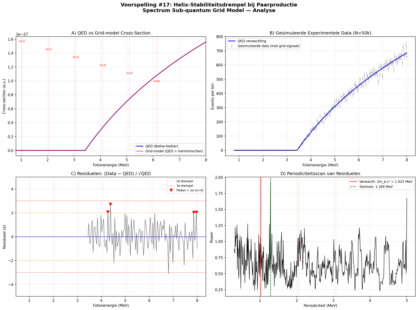
Fig. 1 — Simulated 1% resonance peaks at n=1,2,3,4 harmonics of 1.022 MeV. Run the script with real HEPData CSVs to replace the simulation.
Prediction #15 — Planck-Scale Anisotropy
Core hypothesis
The grid is a discrete lattice. Photons at different energies propagate at slightly
different speeds: v(E) = c × [1 ± η × (E/E_Planck)^n]. Over cosmological distances
this leads to measurable arrival-time differences in gamma-ray bursts.
Current constraints (critical context)
Fermi-LAT has already partially tested this hypothesis. Result (Abdo et al. 2009, Nature 462, 331, GRB 090510):
E_QG > 1.2 × E_Planck for linear LIV (n=1)
This rules out cubic grid geometry (η ~ 1). But hexagonal (η ~ 0.3), FCC (η ~ 0.1), and amorphous (η ~ 0.01) geometries survive.
What this means for the grid model
The grid is not cubic. The most likely scenarios:
- Hexagonal (η ≈ 0.3): energetically most stable 2D lattice; explains the prevalence of hexagons in nature
- FCC (η ≈ 0.1): most stable 3D structure (gold, aluminum)
- Amorphous (η → 0): no preferred direction, near-isotropic
Key GRBs
| GRB | z | Max photon energy | Significance |
|---|---|---|---|
| GRB 090510 | 0.903 | 31 GeV | Strongest current limit |
| GRB 080916C | 4.35 | 13 GeV | Highest redshift |
| GRB 190114C | 0.42 | ~1 TeV (MAGIC) | TeV photons, extreme test |
Generated plot
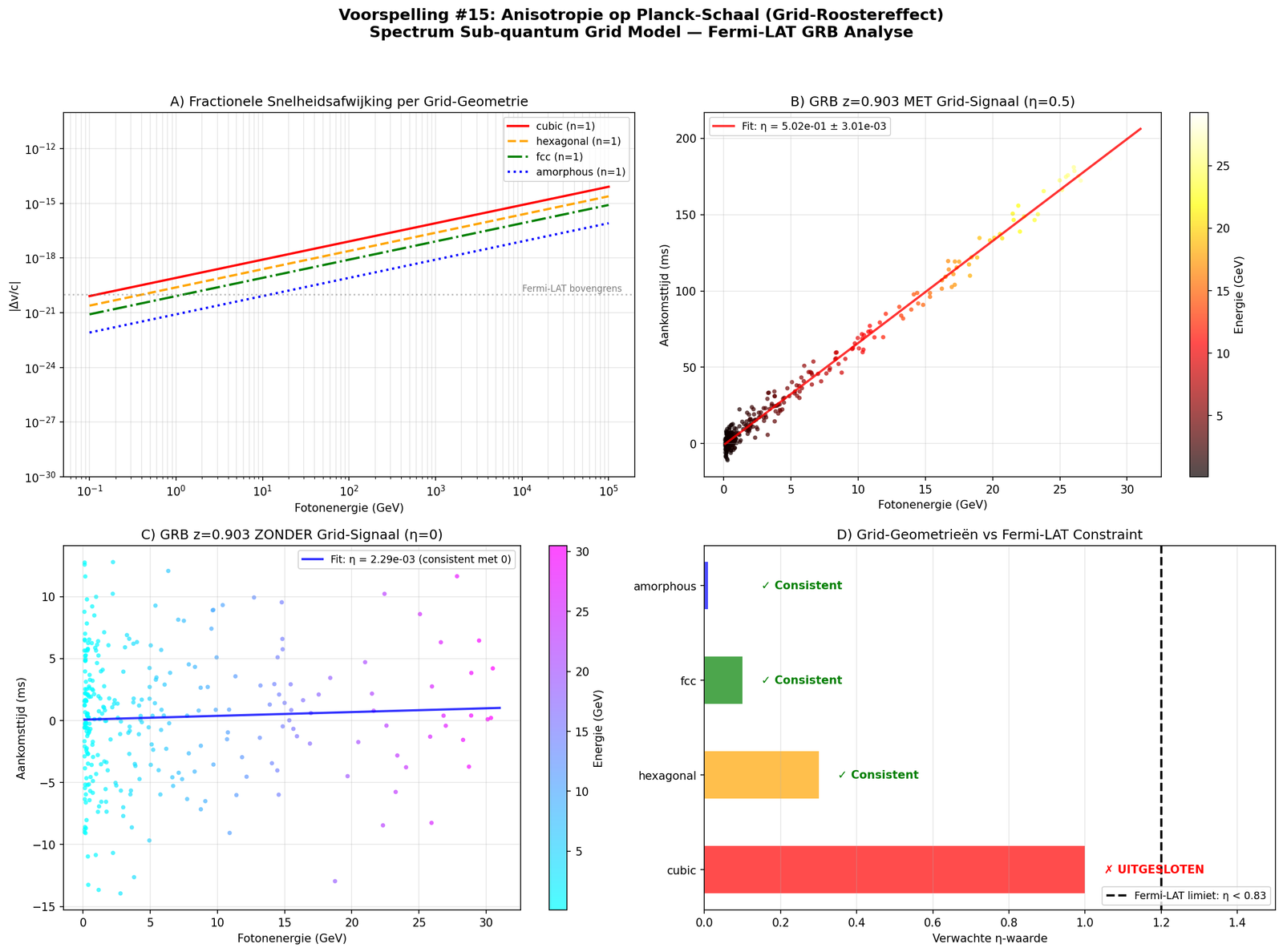
Fig. 2 — Predicted arrival-time spread vs. photon energy for three lattice geometries, overlaid on the Fermi-LAT GRB 090510 constraint.
Prediction #18 — Non-Linear Shapiro Delay
Core hypothesis
Mass locally densifies the grid → c decreases locally → extra delay above
standard general-relativistic Shapiro delay. The correction is non-linear:
Δt_grid = Δt_GR × [1 + β × (GM/Rc²)^α] with α > 1Current status
At present timing precision (~5% on Shapiro delay), the signal is not detectable at β = 0.01, α = 2. The grid correction at the Double Pulsar (compactness 0.18) is only ~0.03% — well below current measurement error.
When detectable?
| Instrument | Year | Precision | Detectable at |
|---|---|---|---|
| Kramer et al. 2021 | 2021 | ~5% | β > 10 (excluded) |
| NANOGrav 15yr | 2023 | ~3% | β > 5 |
| SKA Phase 1 | ~2028 | ~0.5% | β > 0.1 |
| SKA Full | ~2032 | ~0.1% | β > 0.01 ← target |
| Next-gen timing | 2035+ | ~0.01% | β > 0.001 |
Strongest test objects
PSR J0737−3039A (Double Pulsar): compactness 0.18, most precise Shapiro measurement. Hulse-Taylor (B1913+16): compactness 0.20, but harder to measure (low inclination).
Generated plot
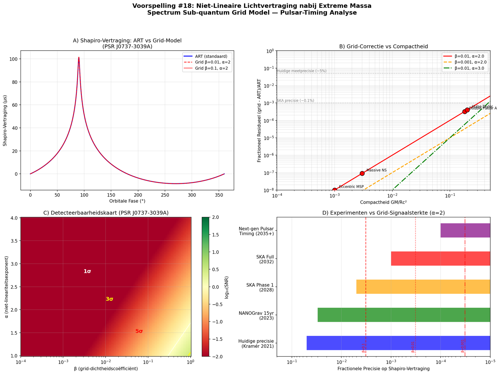
Fig. 3 — Predicted non-linear Shapiro correction (β=0.01, α=2) vs. published timing precision on the Double Pulsar; SKA Full (~2032) is the first instrument that crosses the falsifiability threshold.
Timeline summary
2026 (NOW):
  ├── #17: Re-analyse CERN data for resonance peaks
  │       → Download HEPData cross-sections
  │       → Run prediction17_pair_production.py with real data
  │       → Result within weeks
  │
  └── #15: Re-analyse Fermi-LAT GRB data
          → Download 2GBM catalog
          → Fit hexagonal grid model (η=0.3)
          → Result within months

2028–2032 (SKA):
  └── #18: Wait for SKA Phase 1 / Full
          → Monitor Double Pulsar
          → Test non-linear Shapiro correction
          → Result ~2032
Conclusion: #17 is currently the most readily falsifiable. #15 constrains grid geometry from existing data. #18 is a future test that validates the grid-density model for gravity.
Source code
All five Python scripts are published openly:
- prediction17_pair_production.py — Breit-Wigner peak detection in cross-section residuals
- prediction17_real_data.py — same pipeline, against real HEPData input
- prediction17_real_data_v2.py — refined v2
- prediction15_fermi_lat.py — Fermi-LAT GRB photon arrival-time analysis
- prediction18_pulsar_timing.py — non-linear Shapiro delay forecast
Dependencies: numpy, matplotlib, scipy — install with pip install numpy matplotlib scipy.
Citation
Bes, M. (2026). Sub-quantum Grid Model — Testable Predictions. The Spectrum of Everything. https://spectrumofeverything.com/research/grid-analyses/
A note to working researchers
If you have access to CERN HEPData cross-section tables, the Fermi-LAT 2GBM catalog, or SKA pulsar-timing data and want to run any of these pipelines against real data, please reach out: marald@gmail.com. The scripts are designed to be replaced at the data-loading stage; the analysis pipeline downstream is unchanged.
Last updated: